How to Add a Drop-Down List in Excel

Drop-down lists in Excel make your spreadsheets easier to use. Instead of typing values, users can simply choose from a list. This is useful for data entry, forms, and reports. Here’s a simple guide with steps, pictures, and video resources.

Step 1: Prepare Your List of Options

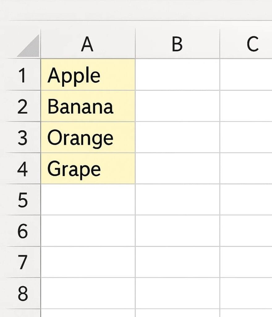
1. Open your Excel workbook.
2. Type the list of items you want in the drop-down into a column or row.
3. Example: In cells A1–A4, type Apple, Banana, Orange, Grape.

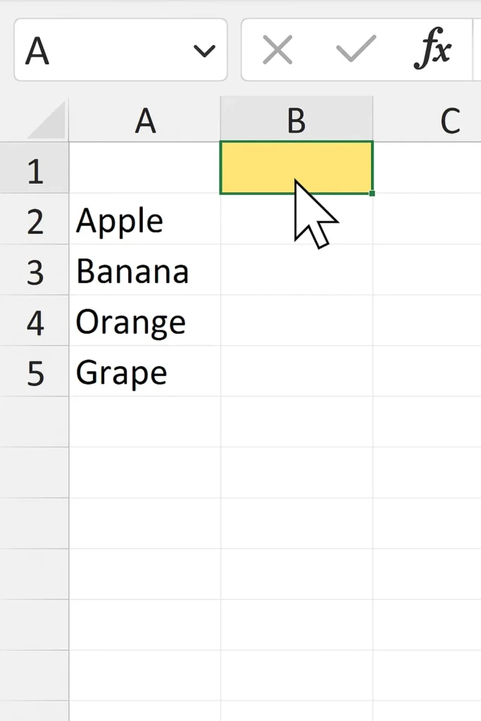
Step 2: Select the Cell for the Drop-Down

• Click on the cell where you want the drop-down menu (example: cell B1).

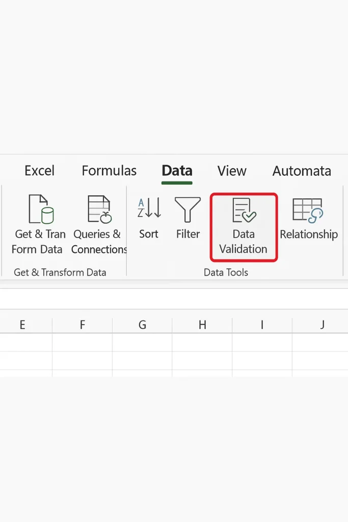
Step 3: Open Data Validation

1. Go to the Data tab in the Ribbon.
2. Click Data Validation (in the Data Tools group).

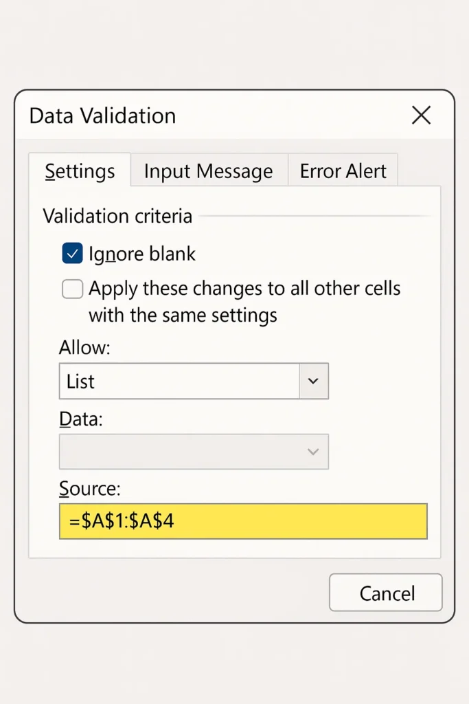
Step 4: Create the Drop-Down

1. In the Data Validation dialog box, under Settings:
   1. Choose List from the “Allow” drop-down.
2. In the Source field, type the cell range containing your list (example: =$A$1:$A$4).
3. Click OK.

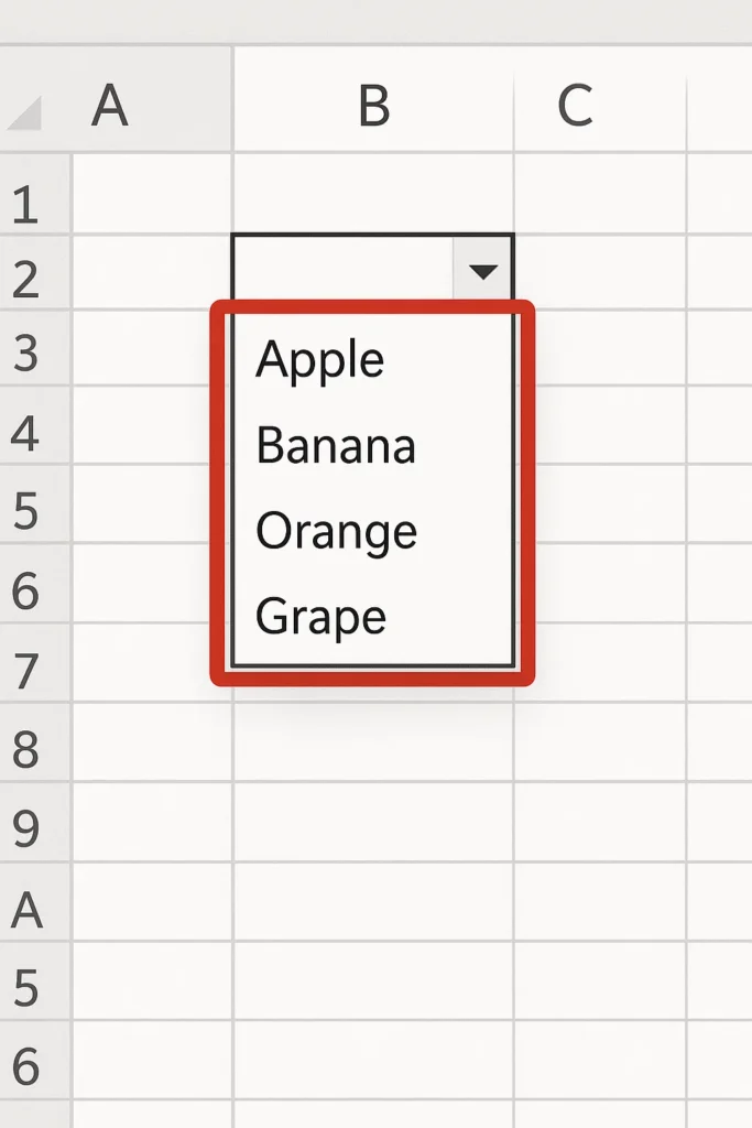
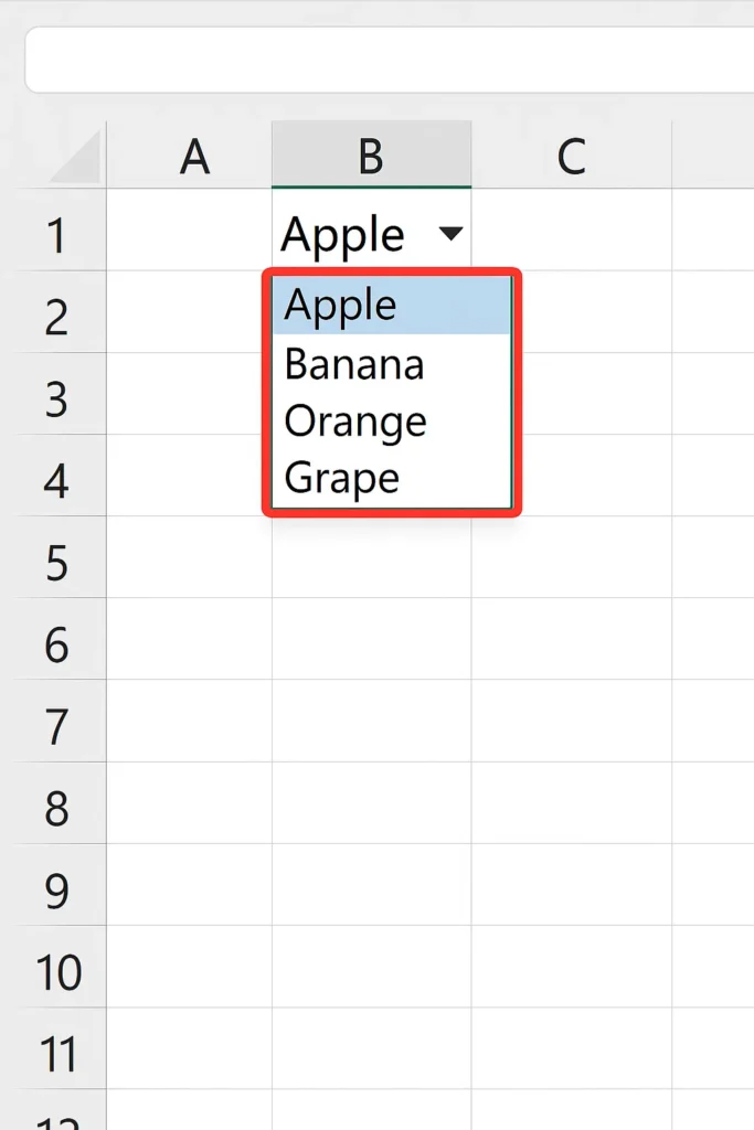
Step 5: Test Your Drop-Down

• Now, click the drop-down arrow in your selected cell (B1).
• You should see your list of fruits.

Bonus Tips

• Multiple Cells: Select multiple cells before adding the drop-down to apply it to all.
• Dynamic Lists: Use a named range for lists that might grow or change.
• Prevent Errors: In the Data Validation dialog, enable “Ignore blank” or add a custom error message.

---

Video Guide (Suggested Embed)

You can embed a YouTube video for your readers:

• How to Create a Drop-Down List in Excel (Excel Campus, YouTube)
• Drop-Down Lists Explained in Excel (Leila Gharani, YouTube)

Final Thoughts

Drop-down lists keep your Excel sheets neat and user-friendly. Whether you’re managing inventory, creating surveys, or building forms, this feature saves time and reduces mistakes.